Mathematical modeling of oxidation process: The oxidation process can be visualized by the following schematic diagram.

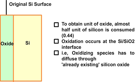
Fig 7.1. Result of oxidation process. A schematic.

 To obtain one unit of silicon dioxide almost half unit of silicon is to be consumed. The oxidation occurs at the silicon and the silicon dioxide interface that is the oxidizing species whether it is oxygen or stream has to diffuse through already existing silicon dioxide. The equations describing the growth of oxides are derived below. The final solution shows that the thickness of the oxide will change with time in a complex manner. At very short times we can neglect certain terms and we see that the thickness is proportional to the time. At longer time, the thickness changes with square root of time.

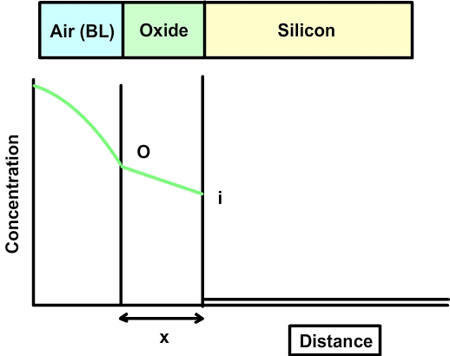
Fig 7.2.  A qualitative plot of concentration of oxidant vs distance.

The concentration of the oxidizing agent (either water or oxygen) will change in the boundary layer (BL) of the gas phase. Let the oxide thickness at any time be ‘x’. The concentration of the species at the outer layer (i.e. oxide and air interface) is given by N0, while the concentration at inner layer (i.e. oxide and silicon interface) is given by Ni.  The diffusion flux, given by Fick’s law, is  . The reaction rate at the interface is given by . i.e. the reaction is first order in oxygen (or water) and zero order in silicon. Under pseudo steady state conditions, the diffusion rate and reaction rate are equal. Hence, the concentration at the interface can be written as

The flux at the steady state is given by
Based on the Avagadro’s number  and the density of oxide, we can calculate the number of molecules of oxide in one unit volume.  It is molecules/cm3. We also know that one mole of oxygen diffusing through the oxide will give one mole of silicon dioxide. On the other hand, in wet oxidation, one mole of steam diffusing through the oxide will give only half a mole of silicon dioxide. Thus, we can relate the flux and the oxide growth rate.
, where
n =  molecules/cm3 for oxygen and  molecules/cm3 for water. The initial condition for the above differential equation is given by  t = 0, x = xi, where xi is the initial thickness of the oxide.

The solution is given by . Here, t is the time corresponding to ‘creating the initial oxide from bare silicon’ and is given

by ,  with . The solution can also be written as .

Note that the values of “A” and “B” depend on the diffusivity and the value of ‘n’. Thus, they are different for wet and dry oxidation. They also vary with temperature.
At short time intervals  and at  long time intervals . Hence, at the short time interval, if we start with the pure silicon, the growth rate of oxide will be in what is known as linear regime. At longer time intervals the growth rate will be slower because the oxidation species has to diffuse through an already existing thickness of oxide, and it will be slower and it is called parabolic regime. In the beginning the growth rate is controlled by the maximum reaction possible (i.e. the kinetic controlled reaction). At later stage, a thick oxide will have formed and the transfer of the species or the diffusion of the species will limit the growth rate. This is called mass transfer controlled growth. The overall implication is that thicker oxide needs more time to grow than thinner oxide. The entire model describing this phenomenon is called Deal-Grove model which was first proposed by Bruce Deal and Andrew Grove. (Andrew Grove was the one of the founders of the Intel Corporation, USA).