|
3.2.3 Diffusivity: A Simple Model
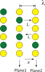
| Figure 3. 1 Schematic of the planes of atoms with arrows showing the cross-movement of species |
As shown in Figure (3.1), a schematic diagram shows atomic planes, illustrating 1-D diffusion of species across the planes .
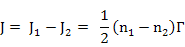
Flux from position (1) to (2) is written as
where n1 is no. of atoms at position (1) and Γ is the jump frequency i.e number of atoms jumping per second (atoms/s)
Similarly, Flux from plane (2) to (1) is expressed as
where n2 is the number of atoms at (2) and Γ is the jump frequency in s-1.
in both the above expressions, factor ½ is there because of equal probability of jump in +x and -x directions.
Now, the net flux, J, can be calculated as
 |
(3.5) |
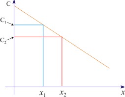
Concentration is defined as
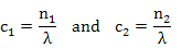 |
| (3.6) |
if area is considered as unit area (=1) and λ is the distance between two atomic planes.
| Figure 3. 2 Schematic diagram showing concentration gradient between two planes of atoms |
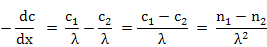
Concentration gradient can be written as (note the minus sign)
 |
(3.7) |
Hence, flux can now be expressed as
where D = ½ λ2 τ with unit cm2/s in 1-D and can easily show to become D = 1/6 λ2 τ in a 3-D cubic co-ordination scenario.
In general, diffusivity can be expressed as
 |
(3.9) |
where γ is governed by the possible number of jumps at an instant and λ is the jump distance and is governed by the atomic configuration and crystal structure.
|