Row Operations and Equivalent Systems

DEFINITION 2.2.1 (Elementary Operations)   The following operations 1, 2 and 3 are called elementary operations.

1. interchange of two equations, say ``interchange the $i^{\mbox{th}}$ and $j^{\mbox{th}}$ equations";

   (compare the system (2.1.2) with the original system.)

2. multiply a non-zero constant throughout an equation, say ``multiply the $k^{\mbox{th}}$ equation by $c \neq 0$ ";

   (compare the system (2.1.5) and the system (2.1.4).)

3. replace an equation by itself plus a constant multiple of another equation, say ``replace the $k^{\mbox{th}}$ equation by $k^{\mbox{th}}$ equation plus $c$ times the $j^{\mbox{th}}$ equation".

   (compare the system (2.1.3) with (2.1.2) or the system (2.1.4) with (2.1.3).)

Remark 2.2.2  

1. In Example 2.1.4, observe that the elementary operations helped us in getting a linear system (2.1.5), which was easily solvable.
2. Note that at Step 1, if we interchange the first and the second equation, we get back to the linear system from which we had started. This means the operation at Step 1, has an inverse operation. In other words, INVERSE OPERATION sends us back to the step where we had precisely started.

So, in Example 2.1.4, the application of a finite number of elementary operations helped us to obtain a simpler system whose solution can be obtained directly. That is, after applying a finite number of elementary operations, a simpler linear system is obtained which can be easily solved. Note that the three elementary operations defined above, have corresponding INVERSE operations, namely,

1. ``interchange the $i^{\mbox{th}}$ and $j^{\mbox{th}}$ equations",
2. ``divide the $k^{\mbox{th}}$ equation by $c \neq 0$ ";
3. ``replace the $k^{\mbox{th}}$ equation by $k^{\mbox{th}}$ equation minus $c$ times the $j^{\mbox{th}}$ equation".

It will be a useful exercise for the reader to IDENTIFY THE INVERSE OPERATIONS at each step in Example 2.1.4.

DEFINITION 2.2.3 (Equivalent Linear Systems)   Two linear systems are said to be equivalent if one can be obtained from the other by a finite number of elementary operations.

The linear systems at each step in Example 2.1.4 are equivalent to each other and also to the original linear system.

LEMMA 2.2.4   Let $C {\mathbf x}= {\mathbf d}$ be the linear system obtained from the linear system $A {\mathbf x}= {\mathbf b}$ by a single elementary operation. Then the linear systems $A {\mathbf x}= {\mathbf b}$ and $C {\mathbf x}= {\mathbf d}$ have the same set of solutions.

Proof. We prove the result for the elementary operation ``the $k^{\mbox{th}}$ equation is replaced by $k^{\mbox{th}}$ equation plus $c$ times the $j^{\mbox{th}}$ equation." The reader is advised to prove the result for other elementary operations.

In this case, the systems $A {\mathbf x}= {\mathbf b}$ and $C {\mathbf x}= {\mathbf d}$ vary only in the $k^{\mbox{th}}$ equation. Let $({\alpha}_1, {\alpha}_2, \ldots, {\alpha}_n)$ be a solution of the linear system $A {\mathbf x}= b.$ Then substituting for ${\alpha}_i$ 's in place of $x_i$ 's in the $k^{\mbox{th}}$ and $j^{\mbox{th}}$ equations, we get

$$a_{k1} {\alpha}_1 + a_{k2} {\alpha}_2 + \cdots a_{kn} {\alpha}_n ... ...d }} \; a_{j1} {\alpha}_1 + a_{j2} {\alpha}_2 + \cdots a_{jn} {\alpha}_n = b_j.$$

Therefore,

$$(a_{k1} + c a_{j1}) {\alpha}_1 + (a_{k2} + c a_{j2}) {\alpha}_2 + \cdots + (a_{kn} + c a_{jn}) {\alpha}_n = b_k + c b_j.$$ (2.2.1)

But then the $k^{\mbox{th}}$ equation of the linear system $C {\mathbf x}= {\mathbf d}$ is

$$(a_{k1} + c a_{j1}) x_1 + (a_{k2} + c a_{j2}) x_2 + \cdots + (a_{kn} + c a_{jn}) x_n = b_k + c b_j.$$ (2.2.2)

Therefore, using Equation (2.2.1), $({\alpha}_1, {\alpha}_2, \ldots, {\alpha}_n)$ is also a solution for the $k^{\mbox{th}}$ Equation (2.2.2).

Use a similar argument to show that if $(\beta_1, \beta_2, \ldots, \beta_n)$ is a solution of the linear system $C {\mathbf x}= {\mathbf d}$ then it is also a solution of the linear system $A {\mathbf x}= {\mathbf b}.$

Hence, we have the proof in this case. height6pt width 6pt depth 0pt

Lemma 2.2.4 is now used as an induction step to prove the main result of this section (Theorem 2.2.5).

THEOREM 2.2.5   Two equivalent systems have the same set of solutions.

Proof. Let $n$ be the number of elementary operations performed on $A {\mathbf x}= {\mathbf b}$ to get $C {\mathbf x}= {\mathbf d}.$ We prove the theorem by induction on $n.$

If $n = 1,$ Lemma 2.2.4 answers the question. If $n > 1,$ assume that the theorem is true for $n = m.$ Now, suppose $n = m+1.$ Apply the Lemma 2.2.4 again at the ``last step" (that is, at the $(m+1)^{\mbox{th}}$ step from the $m^{\mbox{th}}$ step) to get the required result using induction. height6pt width 6pt depth 0pt

Let us formalise the above section which led to Theorem 2.2.5. For solving a linear system of equations, we applied elementary operations to equations. It is observed that in performing the elementary operations, the calculations were made on the COEFFICIENTS (numbers). The variables $x_1, x_2, \ldots, x_n$ and the sign of equality (that is, $\lq\lq =''$ ) are not disturbed. Therefore, in place of looking at the system of equations as a whole, we just need to work with the coefficients. These coefficients when arranged in a rectangular array gives us the augmented matrix $[ A \; \; {\mathbf b}].$

DEFINITION 2.2.6 (Elementary Row Operations)   The elementary row operations are defined as:

1. interchange of two rows, say ``interchange the $i^{\mbox{th}}$ and $j^{\mbox{th}}$ rows", denoted $R_{ij};$
2. multiply a non-zero constant throughout a row, say ``multiply the $k^{\mbox{th}}$ row by $c \neq 0$ ", denoted $R_k(c);$
3. replace a row by itself plus a constant multiple of another row, say ``replace the $k^{\mbox{th}}$ row by $k^{\mbox{th}}$ row plus $c$ times the $j^{\mbox{th}}$ row", denoted $R_{kj}(c).$

EXERCISE 2.2.7   Find the INVERSE row operations corresponding to the elementary row operations that have been defined just above.

DEFINITION 2.2.8 (Row Equivalent Matrices)   Two matrices are said to be row-equivalent if one can be obtained from the other by a finite number of elementary row operations.

EXAMPLE 2.2.9   The three matrices given below are row equivalent.
$\begin{bmatrix}0 & 1 & 1 & 2 \\ 2 & 0 & 3 & 5 \\ 1 & 1 & 1 & 3 \end{bmatrix} \... ... 0 & \frac{3}{2} & \frac{5}{2} \\ 0 & 1 & 1 & 2 \\ 1 & 1 & 1 & 3 \end{bmatrix}.$

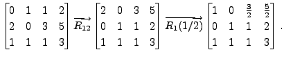
Whereas the matrix 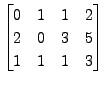$\begin{bmatrix}0 & 1 & 1 & 2 \\ 2 & 0 & 3 & 5 \\ 1 & 1 & 1 & 3 \end{bmatrix}$ is not row equivalent to the matrix $\begin{bmatrix}1 & 0 & 1 & 2 \\ 0 & 2 & 3 & 5 \\ 1 & 1 & 1 & 3 \end{bmatrix}.$