4.5.3 Dipolar or Orientation Polarization
In case of dipolar polarization, we have materials where the dipoles are present independent of each other, i.e. they don’t interact and they can be rotated freely by an applied field unlike in case of ionic polarization.
One such example is water where each H2O molecule has a dipole moment and these dipole moments are free to rotate and can have any orientation with respect to neighbouring molecules. Due to the ability of molecules to move around randomly, liquids like water have very limited dipolar polarization contribution despite having a permanent dipole moment for each molecule.
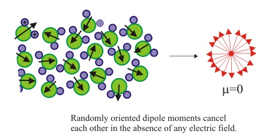
A two dimensional image of water molecules is shown below which should remain almost similar at any instant. Arrows depict the direction of dipole moment associated with each molecule.
| Figure 4.12 Dipoles in a polar material |
It is quite obvious by looking at the figure that in the absence of an applied field, all the moments are randomly distributed (huge number for even a small amount of water, say 10 ml) and net dipole moment would be zero.
Now when we apply an external electric field say parallel to the paper along +X- axis as shown below, the dipoles would tend to align with the applied field to lower their electrostatic energy and lead to minimum dipole energy (basically the positive end of the dipole would like to join the negative end of the applied field).
For instance, water does have a pretty large dielectric constant of ~80 which means that there is obviously some orientation along the field.
Exercise
You can show it to yourself that this dielectric constant is several orders of magnitude smaller than for fully oriented dipole moments at some normal field strengths (see here for solution).
In reality, the tendency of dipoles to orient along into the field direction will be counteracted by random collisions between molecules, a process driven by the thermal energy ‘kT’ at a temperature ‘T’. Moreover, the dipole containing molecules move around at all times due to thermal energy and the associated entropy i.e. disorder.
So, basically when we apply an external field, there is a competition between field induced order and thermal driven disorder. The Later prevails in liquids more than in solids. Hence, perfect alignment of dipoles would be possible only at very low temperature and possibly in solid crystals.
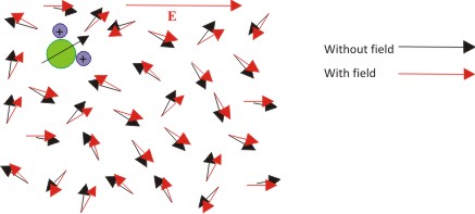
As a result of intermolecular collisions and thermally induced random movement, the dipoles do not completely align themselves along the field unless the field is extremely high. So basically, the configuration of dipoles looks something like shown below.
| Figure 4.13 Effect of electric field on the dipole orientation |
This basically highlights that the orientation of all the dipoles is just a little bit shifted towards the field direction leading to an average non-zero dipole moment in the direction of the applied electric field.
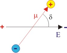
Thermodynamically speaking, we will minimize the free energy, G which is equal to H – TS where H is the internal energy and S is the entropy. So for this, now we take the following configuration where the charge dipole of an molecule makes an angle, θ, to the applied field.
| Figure 4.14 2-D schematic diagram of a charge dipole aligned with respect to applied field |
The internal energy, U, of a dipole depends on its orientation with respect to the applied field, i.e. it is function of θ.
U is minimum when the dipole is completely aligned with the field i.e.θ = 0 and maximum if θ = 180o.
The energy U(θ) of a dipole with dipole moment, μ under an applied field, E, can be written as
 |
(4.41) |
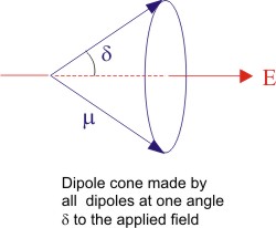
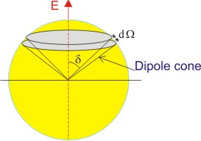
What it means in 3-D world is that we would have a cone of dipoles making an angle θ around the applied field E which points along the axis of the cone as shown below. The total internal energy of the whole material would be the sum of internal energies of all these cones.
| Figure 4.15 Schematic representation of dipoles around the electric field |
Now we need to calculate the number of dipoles at an angle θ, N(θ) which can then be multiplied with the energy for that θ and then be integrated between θ ranging from 0 to 180° to give us the total internal energy. However, to calculate the free energy, we also need to calculate the entropy, S, which is not very straightforward.
This is where Boltzman statistics (from classical thermodynamics) rescues us which allows us to work out the minimum of the free energy using a distribution function.
We treat our system, to a good approximation, as a classical system containing a number of independent entities (the dipoles), occupying various energies as determined by their angle w.r.t. applied field. The distribution of these dipoles at various energies can be expressed by a distribution function in such a manner that it minimizes the free energy of the system.
Now, at a given temperature, T, the number of dipoles with energy U can expressed as
 |
(4.42) |
where A is a constant and kB is Boltzmann constant.
Equation (4.42) provides us the number of dipoles in a cone as shown above.
Now, we should calculate the component of the dipole moment parallel to the applied field using the solid angle dΩ for a unit sphere in the segment between θ and θ + dθ.
| Figure 4.16 Spherical representation of dipoles |
This implies that the number of dipoles between θ and θ + dθ is equal to N(U( θ)).d θ.
The total dipole moment is nothing but the sum of the components of the dipole moments in direction of applied field i.e.
 |
(4.43) |
The average dipole moment, <μE>, is calculated by adding up the contributions from all the solid angles i.e.
 |
(4.44) |
The incremental solid can be expressed as
 |
(4.45) |
which together with (4.42) yields
 |
(4.46) |
To solve this equation, we make substitutions as β = (μE/kBT) and x = cos θ in the above equation which yields
 |
(4.47) |
or rather
 |
(4.48) |
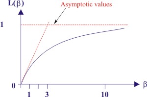
where L(β) = Langevin function, named after Paul Langevin, and is defined as
 |
(4.49) |
The function cot h(x) is nothing but (ex + e-x) / (ex - e-x). We won’t go into details of L(x) except that it is not an easy function to deal with and L(x) values are between 0 and 1 for our purposes.
Langevin function is plotted as shown below.
| Figure 4.17 Schematic plot of Langevin function |
As we can see, for large values of β (i.e. large electric fields or very low temperatures, close to 0 K),
 |
(4.50) |
while for small values of (β< 1) i.e. nominal fields and higher temperatures, the slope is 1/3 for β → 0 and hence the Langevin function is approximated by
 |
(4.51) |
In general, β is always much smaller than one i.e.β << 1.
As a result, the induced dipole moment, often called as Langevin - Debye equation is given as
 |
(4.52) |
Where αd is dipolar polarizability. Now, the average polarization is
 |
(4.53) |
These equations hold pretty well for small values of μ and E and/or large enough T which we can presume as normal conditions.
In fact when fields are very high and temperature is very low (i.e. minimizing the randomization), all the dipoles would be parallel to the applied field and then the average dipole moment would be equal to the theoretical dipole moment.
Equation (4.52) also shows the temperature dependence of dipolar polarizability as μ = α, unlike in the case of electronic and ionic polarization.
|